import pandas as pd
from sqlalchemy import create_engine

connection_string = "mysql+mysqlconnector://tcrd@tcrd.kmc.io/tcrd540"
engine = create_engine(connection_string)

# Get targets in Tclin and Tchem
query_target = """
  SELECT id, name, tdl, fam, famext
  FROM target
  WHERE tdl IN ('Tclin','Tchem')
"""
target = pd.read_sql(query_target, con=engine)

# Get Uniprot ids
query_protein = "SELECT id, uniprot, family FROM protein"
protein = pd.read_sql(query_protein, con=engine)

# Get compound activities
query_cmpd_activity = """
  SELECT id, target_id, act_value
  FROM cmpd_activity
"""

cmpd_activity = pd.read_sql(query_cmpd_activity, con=engine)A common goal in early drug discovery is to prioritize targets that not only have known active compounds but also have experimentally determined protein structures in the Protein Data Bank (PDB). This sets the stage for more in-depth analyses such as structure-based drug design (SBDD) and structure-activity relationship (SAR).
Here, we combine two key data sources:
- Pharos/TCRD (Target Central Resource Database) – an NIH-funded knowledgebase containing data for human targets, their associated ligands/compounds, and many annotations such as gene families and drug development levels (Tclin, Tchem, etc.).
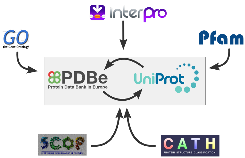
- SIFTS (Structure Integration with Function, Taxonomy and Sequence) – the EBI’s resource mapping UniProt accessions to PDB structures, as well as other databases such as GO, InterPro, Pfam, CATH, SCOP, and PubMed.
By merging these data, we can quickly identify human protein targets that (A) meet a minimum threshold of known active compounds (≥15 in this example), and (B) have PDB structures available for structure-based work.
Below is a brief, self-contained workflow that:
- Connects to Pharos via MySQL to retrieve targets in the Tclin/Tchem development levels.
- Collects compound-activity counts.
- Retrieves UniProt-PDB mappings from SIFTS.
- Joins the data, flags targets that have ≥15 active compounds and at least one PDB structure.
- Explores target families and visualizes the final set.
You can adapt this workflow to explore deeper aspects of SAR, binding modes, or structure-based design.
Getting Target Data from Pharos
First, we connect to the Pharos database with the help of SQLAlchemy and read the necessary tables into Pandas DataFrames.
Here are the datasets that we obtained:
target.head()| id | name | tdl | fam | famext | |
|---|---|---|---|---|---|
| 0 | 2 | 14-3-3 protein eta | Tchem | None | None |
| 1 | 3 | 14-3-3 protein theta | Tchem | None | None |
| 2 | 23 | 3 beta-hydroxysteroid dehydrogenase/Delta 5-->... | Tchem | Enzyme | 3-beta-HSD |
| 3 | 26 | 5-hydroxytryptamine receptor 2B | Tclin | GPCR | GPCR |
| 4 | 27 | 5-hydroxytryptamine receptor 2C | Tclin | GPCR | GPCR |
protein.head()| id | uniprot | family | |
|---|---|---|---|
| 0 | 1 | P62258 | Belongs to the 14-3-3 family. |
| 1 | 2 | Q04917 | Belongs to the 14-3-3 family. |
| 2 | 3 | P27348 | Belongs to the 14-3-3 family. |
| 3 | 4 | P30443 | Belongs to the MHC class I family. |
| 4 | 5 | P04439 | Belongs to the MHC class I family. |
cmpd_activity.head()| id | target_id | act_value | |
|---|---|---|---|
| 0 | 1 | 3006 | 7.60 |
| 1 | 2 | 3006 | 7.68 |
| 2 | 3 | 3006 | 7.77 |
| 3 | 4 | 3006 | 7.80 |
| 4 | 5 | 3006 | 7.89 |
Filtering targets with more than 15 active compounds
actives_count = (
    cmpd_activity
    .groupby('target_id', as_index=False)
    .agg(num_actives=('id','count'))
)

# Merge with the target table
target = target.merge(actives_count,
                      left_on='id',
                      right_on='target_id',
                      how='left')

# Keep only targets with >= 15 active compounds
target = target[target['num_actives'] >= 15]
At this point, we have a table of Tclin/Tchem targets that each have at least 15 active compounds recorded in Pharos.
Read SIFTS Mappings
The SIFTS PDB chain to UniProt mappings were downloaded from their ftp site.
import requests
import tempfile
from typing import Dict, List

sifts_url = "https://ftp.ebi.ac.uk/pub/databases/msd/sifts/flatfiles/csv/pdb_chain_uniprot.csv.gz"

dtypes: Dict[str, str] = {
    'PDB': str,
    'CHAIN': str,
    'SP_PRIMARY': str,
    'RES_BEG': int,
    'RES_END': int,
    'PDB_BEG': str,  # Keep as string since it may contain insertion codes
    'PDB_END': str,  # Keep as string since it may contain insertion codes
    'SP_BEG': int,
    'SP_END': int
}

with tempfile.TemporaryDirectory() as tmpdirname:
    response = requests.get(sifts_url)
    gz_file_path = f"{tmpdirname}/pdb_chain_uniprot.csv.gz"
    with open(gz_file_path, "wb") as gz_file:
        gz_file.write(response.content)  # Raw compressed bytes
    # Read the gzipped CSV with pandas
    sifts_data = pd.read_csv(
        gz_file_path,
        compression="gzip",
        comment="#",
        dtype=dtypes
    )

# Rename the columns
sifts_data.rename(
    columns={
        "PDB": "pdb",
        "CHAIN": "chain_id",
        "SP_PRIMARY": "uniprot",
        "RES_BEG": "res_beg",
        "RES_END": "res_end",
        "PDB_BEG": "pdb_res_beg",
        "PDB_END": "pdb_res_end",
        "SP_BEG": "uniprot_res_beg",
        "SP_END": "uniprot_res_end",
    },
    inplace=True
)

sifts_data.head(5)| pdb | chain_id | uniprot | res_beg | res_end | pdb_res_beg | pdb_res_end | uniprot_res_beg | uniprot_res_end | |
|---|---|---|---|---|---|---|---|---|---|
| 0 | 101m | A | P02185 | 1 | 154 | 0 | 153 | 1 | 154 |
| 1 | 102l | A | P00720 | 1 | 40 | 1 | 40 | 1 | 40 |
| 2 | 102l | A | P00720 | 42 | 165 | 41 | NaN | 41 | 164 |
| 3 | 102m | A | P02185 | 1 | 154 | 0 | 153 | 1 | 154 |
| 4 | 103l | A | P00720 | 1 | 40 | 1 | NaN | 1 | 40 |
Note
The SIFTS pdb_chain_uniprot.csv file provides mappings between UniProt accessions and PDB structure chains.
It comes with three sets of residue ranges:
RES_BEG/RES_END: Residue numbers as listed in the SEQRES records of the PDB file.- They represent sequential numbering from 1 to n, of the full structure sequence as intended by the author, including unresolved residues.
PDB_BEG/PDB_END: Residue numbers as they appear in the ATOM records of the PDB file.- May include insertion codes (e.g., 25A, 25B).
- Can have non-sequential jumps due to missing residues or unresolved regions.
- Reflect only the resolved residues with atomic coordinates.
SP_BEGandSP_END: Residue numbers in the canonical UniProt sequence.
For this simple analysis, we only care whether a target has at least one PDB structure, so we can use the pdb (PDB) and uniprot (SP_PRIMARY) columns, but if we wanted to do a structure-based analysis and download the associated PDBs, we could use the residue-level mappings to identify the exact ranges of our PDB that we need to extract, as well as identify any missing residues that may need to be filled.
Now, we can group the SIFTS data by UniProt ID and get a list of unique PDB IDs for each target:
# Group by uniprot_id and get unique PDB IDs
uniprot_to_pdb = (
    sifts_data
    .groupby("uniprot", as_index=False)
    .agg(pdb_ids=("pdb", lambda x: ';'.join(x.unique())))
)
uniprot_to_pdb.head(5)| uniprot | pdb_ids | |
|---|---|---|
| 0 | A0A003 | 6kv9;6kvc |
| 1 | A0A009I821 | 7m4w;7m4x;7m4y;7m4z;7ryf;7ryg;7ryh;7uvv;7uvw;7... |
| 2 | A0A009IHW8 | 7uwg;7uxu;8g83 |
| 3 | A0A009PZ93 | 9kbq |
| 4 | A0A009QSN8 | 6v39;6v3a;6v3b;6v3d |
Merging Target Data with SIFTS
Since our target table has a corresponding protein table (linked by protein.id == target.id in TCRD) and each protein row has a UniProt ID, we can merge the two, and then merge with SIFTS on the UniProt accession:
# Filter the protein table to only those in our target set
protein_subset = protein[protein.id.isin(target.id)]

# Merge target and protein by TCRD 'id'
merged_df = target.merge(protein_subset, left_on='id', right_on='id', how='left')

# Merge SIFTS data
merged_df = merged_df.merge(uniprot_to_pdb, left_on='uniprot', right_on='uniprot', how='left')

# Rename columns for clarity
merged_df.rename(columns={'fam': 'target_family',
                   'tdl': 'target_dev_level'}, inplace=True)

merged_df['target_family'] = merged_df['target_family'].fillna('None', inplace=False)

# Mark whether a target has at least one known PDB structure
merged_df['has_pdb'] = ~merged_df['pdb_ids'].isna()

merged_df.head()| id | name | target_dev_level | target_family | famext | target_id | num_actives | uniprot | family | pdb_ids | has_pdb | |
|---|---|---|---|---|---|---|---|---|---|---|---|
| 0 | 26 | 5-hydroxytryptamine receptor 2B | Tclin | GPCR | GPCR | 26.0 | 777.0 | P41595 | Belongs to the G-protein coupled receptor 1 fa... | 4ib4;4nc3;5tud;5tvn;6drx;6dry;6drz;6ds0;7srq;7... | True |
| 1 | 27 | 5-hydroxytryptamine receptor 2C | Tclin | GPCR | GPCR | 27.0 | 1612.0 | P28335 | Belongs to the G-protein coupled receptor 1 fa... | 6bqg;6bqh;8dpf;8dpg;8dph;8dpi;8zmf | True |
| 2 | 30 | 5'-nucleotidase | Tchem | Enzyme | None | 30.0 | 23.0 | P21589 | Belongs to the 5'-nucleotidase family. | 4h1s;4h1y;4h2b;4h2f;4h2g;4h2i;6hxw;6s7f;6s7h;6... | True |
| 3 | 36 | Amyloid-beta A4 protein | Tchem | None | None | 36.0 | 440.0 | P05067 | Belongs to the APP family. | 1aap;1amb;1amc;1aml;1ba4;1ba6;1bjb;1bjc;1brc;1... | True |
| 4 | 37 | Adenosine receptor A1 | Tclin | GPCR | GPCR | 37.0 | 1550.0 | P30542 | Belongs to the G-protein coupled receptor 1 fa... | 5n2s;5uen;6d9h;7ld3;7ld4 | True |
Visualizing the Data
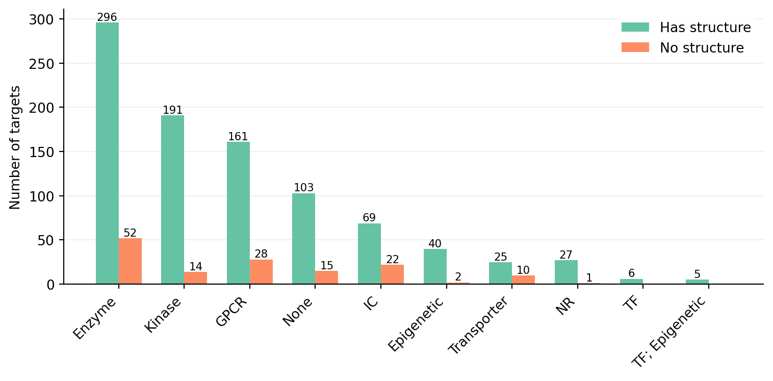
Here, we visualize the count of targets with and without PDB structures, as well as the counts by target family.
Plotting code
import matplotlib.pyplot as plt
import seaborn as sns
import numpy as np
from typing import Tuple

# Set global style

def plot_overall_pdb_counts(df: pd.DataFrame) -> Tuple[plt.Figure, plt.Axes]:
    """
    Plot the number of targets with and without PDB structures.
    """
    total = len(df)
    counts = df['has_pdb'].value_counts()
    percentages = (counts / total * 100).round(1)

    fig, ax = plt.subplots(figsize=(6, 4))
    width = 0.6
    x = np.arange(2)
    colors = ['#66c2a5', '#fc8d62']
    bars = ax.bar(x, counts.values, width, color=colors, zorder=2)

    for bar in bars:
        height = bar.get_height()
        pct = (height/total * 100).round(1)
        ax.text(bar.get_x() + bar.get_width()/2, height, f'{int(height)}\n({pct}%)', ha='center', va='bottom', size=9)

    ax.set_xticks(x)
    ax.set_xticklabels(['Has structure', 'No structure'])
    ax.set_ylabel('Number of targets')
    ax.yaxis.grid(True, linestyle='-', alpha=0.2, zorder=1)
    ax.xaxis.grid(False)
    ax.spines['top'].set_visible(False)
    ax.spines['right'].set_visible(False)
    plt.tight_layout()

    return fig, ax

def plot_pdb_counts_by_family(df: pd.DataFrame) -> Tuple[plt.Figure, plt.Axes]:
    """
    Plot the number of targets with and without PDB structures, grouped by target family.
    """
    family_counts = df.groupby(['target_family', 'has_pdb']).size().unstack(fill_value=0)
    family_totals = family_counts.sum(axis=1)
    family_percentages = (family_counts.div(family_totals, axis=0) * 100).round(1)
    family_counts = family_counts.loc[family_counts.sum(axis=1).sort_values(ascending=False).index]

    fig, ax = plt.subplots(figsize=(8, 4))
    width = 0.35

    x = np.arange(len(family_counts.index))
    bars1 = ax.bar(x - width/2, family_counts[True], width, label='Has structure', color='#66c2a5', zorder=2)
    bars2 = ax.bar(x + width/2, family_counts[False], width, label='No structure', color='#fc8d62', zorder=2)

    def add_value_labels(bars):
        for bar in bars:
            height = bar.get_height()
            if height > 0:
                    ax.text(bar.get_x() + bar.get_width()/2, height, f'{int(height)}', ha='center', va='bottom', fontsize=8)

    add_value_labels(bars1)
    add_value_labels(bars2)

    ax.set_xticks(x)
    ax.set_xticklabels(family_counts.index, rotation=45, ha='right')
    ax.set_ylabel('Number of targets')
    ax.yaxis.grid(True, linestyle='-', alpha=0.2, zorder=1)
    ax.xaxis.grid(False)
    ax.spines['top'].set_visible(False)
    ax.spines['right'].set_visible(False)
    ax.legend(loc='upper right', frameon=True, facecolor='white', framealpha=0.9, edgecolor='none')
    plt.tight_layout()

    return fig, ax
fig, ax = plot_overall_pdb_counts(merged_df)
plt.show()
fix, ax = plot_pdb_counts_by_family(merged_df)
plt.show()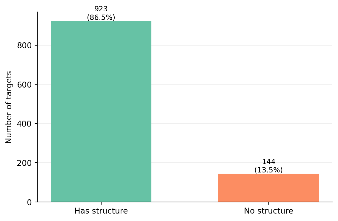
Conclusion
This is a basic example of how we can combine data from Pharos and SIFTS to identify targets with known active compounds and available PDB structures. There are many additional filters and considerations we could apply depending on our specific research questions and goals.
For example, bringing in additional data from the PDB to filter the structures based on resolution, completeness, or other structural features could help refine our target selection further.