---
title: "Extracting Room Boundaries from 3D Scans"
description: |
Using RANSAC and NDT-RANSAC to detect walls from iPhone photogrammetry scans
and extract clean floor plan polygons.
date: "2026-01-18"
categories:
- Python
- computational-geometry
- 3D-reconstruction
format:
html:
code-tools:
source: true
code-fold: true
code-summary: "Show code"
lightbox: true
code-annotations: hover
execute:
echo: true
warning: false
freeze: true
bibliography: references.bib
---
This week I've been working on extracting room boundaries from 3D mesh scans. It is a bit of an ADHD-fueled rabbit hole, but long story short, we moved to a new apartment, and I was wondering if I could use 3D virtual modeling to plan how we are going to lay out our furniture. There's apps out there that scan rooms pretty accurately using LIDAR + ARKit on iPhones (e.g. Apple's [RoomPlan API](https://developer.apple.com/augmented-reality/roomplan/)), but I don't have an iPhone with Lidar, and I wasn't too happy with any of the apps.
The goal: take a noisy point cloud from an iPhone photogrammetry scan (I used the Polycam app with a free trial and exported an OBJ file) and produce a clean polygon representing the room's floor plan.
## The Problem
Given a 3D mesh of a room, I need to:
1. Detect the walls, floor, and ceiling
2. Extract the room's 2D boundary polygon
3. Handle real-world messiness: furniture, alcoves, doorways, windows, mirrors, and other scanning artifacts that cause noise and holes in the mesh.
### Key Terms
Before diving in, some definitions for readers unfamiliar with computational geometry:
- **Point cloud**: A set of 3D points (x, y, z) representing surfaces scanned by a sensor
- **Normal vector**: A unit vector perpendicular to a surface, indicating which way it "faces"
- **Inliers/Outliers**: Points that do/don't fit a proposed model (e.g., points on vs. off a plane)
- **Convex hull**: The smallest convex shape containing all points - imagine stretching a rubber band around pins
- **CCW (Counter-Clockwise) ordering**: When creating a convex hull, the convention is that vertices are listed so that walking along edges keeps the interior on your left
Here's what the raw data looks like - a point cloud colored by height:
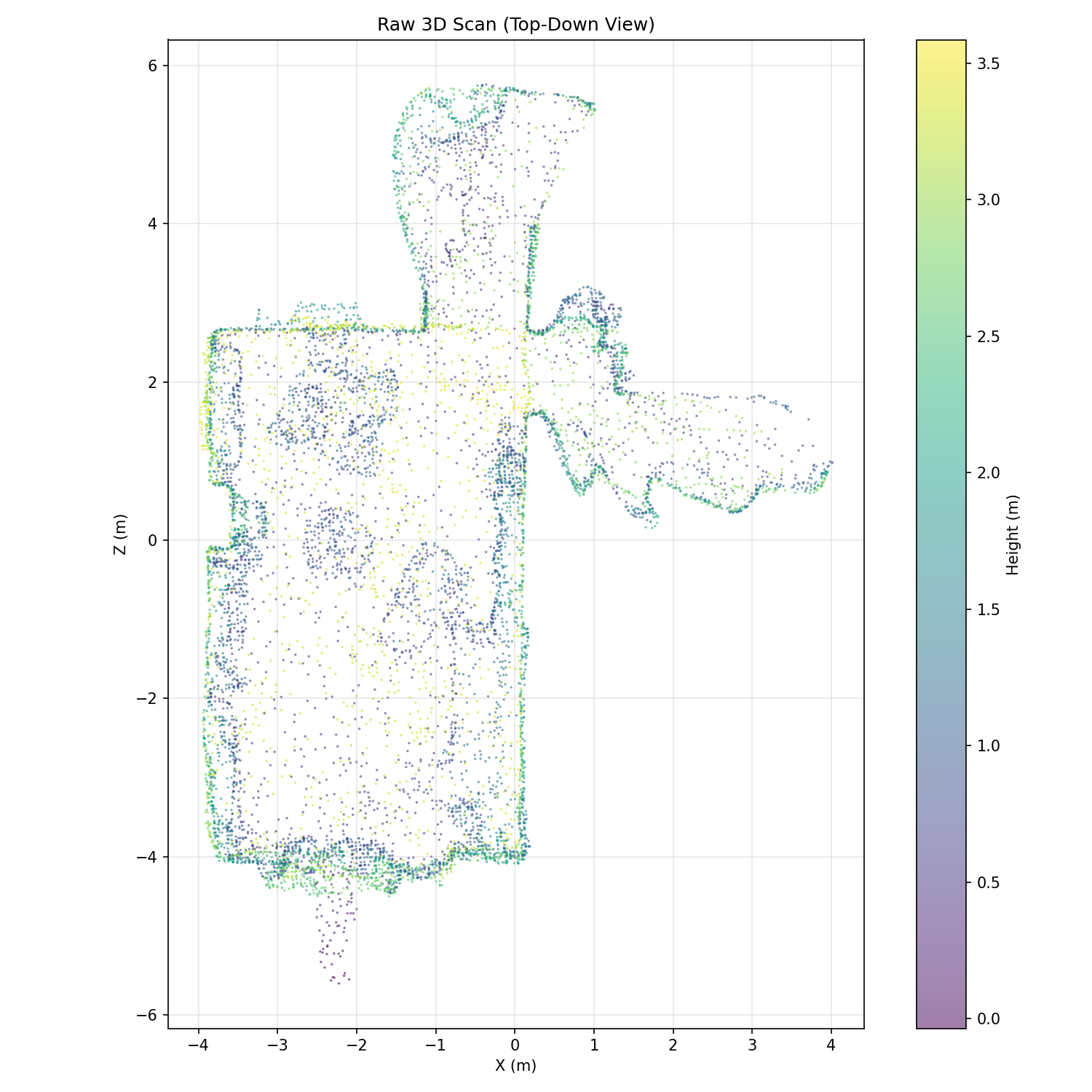{fig-cap="Raw point cloud from a photogrammetry scan of my living room. Yellow/green points are ceiling height, purple points are floor level. The room shape is visible, but extracting a clean boundary is non-trivial. Density from the incompletely scanned hallway and windows makes it more complex, and I find that it may be better to remove that density manually before running the algorithm."}
## Approach: Multi-Plane RANSAC
The foundational algorithm for this task is **RANSAC** (Random Sample Consensus) [@fischler1981]. It is essentially a kind of Monte-Carlo algorithm that repeatedly samples minimal subsets of the data and keeps the model that explains the most data.
### Standard RANSAC for Plane Detection
For plane detection, the algorithm works as follows:
1. **Sample**: Pick 3 random points - the minimum needed to define a plane
2. **Hypothesize**: Fit a plane through these 3 points using the equation $ax + by + cz + d = 0$
3. **Score**: Count inliers - points within distance threshold $\varepsilon$ of the plane
4. **Iterate**: Repeat N times, keep the plane with most inliers
5. **Refine**: Refit the plane using all inliers (not just the 3 samples)
6. **Remove & repeat**: Delete inliers from point cloud, find next plane
Here's the core RANSAC implementation:
```{python}
#| label: ransac-core
import numpy as np
from dataclasses import dataclass
from typing import Optional
@dataclass
class DetectedPlane:
"""A plane detected via RANSAC."""
normal: np.ndarray # Unit normal vector (3,)
point: np.ndarray # Point on plane (3,)
inlier_indices: np.ndarray
inlier_count: int
@property
def d(self) -> float:
"""Plane equation: n·x + d = 0, so d = -n·point."""
return -np.dot(self.normal, self.point)
def ransac_plane(
points: np.ndarray,
threshold: float = 0.02,
iterations: int = 200,
min_inliers: int = 100
) -> Optional[DetectedPlane]:
"""
Single-plane RANSAC with least-squares refinement.
Args:
points: (N, 3) point cloud.
threshold: Distance threshold for inliers (meters).
iterations: Number of RANSAC iterations.
min_inliers: Minimum inliers for a valid plane.
"""
n_points = len(points)
if n_points < 3:
return None
best_inlier_count = 0
best_inlier_mask = None
best_normal = None
best_point = None
for _ in range(iterations):
# Sample 3 random points
idx = np.random.choice(n_points, 3, replace=False) # <1>
p1, p2, p3 = points[idx]
# Compute normal via cross product
v1 = p2 - p1
v2 = p3 - p1
normal = np.cross(v1, v2) # <2>
norm = np.linalg.norm(normal)
if norm < 1e-8: # Collinear points
continue
normal /= norm
# Compute distances to plane
dists = np.abs(np.dot(points - p1, normal)) # <3>
inlier_mask = dists < threshold
count = np.count_nonzero(inlier_mask)
if count > best_inlier_count:
best_inlier_count = count
best_inlier_mask = inlier_mask
best_normal = normal
best_point = p1
if best_inlier_count < min_inliers:
return None
# Refine with least-squares on inliers
inlier_points = points[best_inlier_mask]
centroid = np.mean(inlier_points, axis=0)
centered = inlier_points - centroid
_, _, vh = np.linalg.svd(centered) # <4>
refined_normal = vh[-1]
return DetectedPlane(
normal=refined_normal / np.linalg.norm(refined_normal),
point=centroid,
inlier_indices=np.where(best_inlier_mask)[0],
inlier_count=best_inlier_count
)
```
1. The minimum number of points to define a plane in 3D
2. Cross product gives the normal perpendicular to both edge vectors
3. Signed distance: $d = |(p - p_0) \cdot \mathbf{n}|$
4. SVD gives the best-fit plane normal as the last row of $V^T$
The distance formula measures the **perpendicular** distance from a point to the plane:
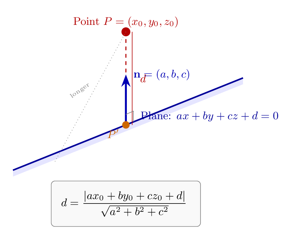{fig-cap="The vector $\\mathbf{n} = (a, b, c)$ is the plane's unit normal. The distance from point $P$ to the plane is the projection of $(P - P_0)$ onto $\\mathbf{n}$."}
### How Many Iterations?
The number of iterations N needed depends on the inlier ratio. If fraction $w$ of points are inliers, the probability of picking 3 good points is $w^3$. To achieve 99% confidence:
$$N = \frac{\log(1 - 0.99)}{\log(1 - w^3)}$$
```{python}
#| label: ransac-iterations
import numpy as np

def ransac_iterations_needed(inlier_ratio: float, confidence: float = 0.99) -> int:
    """Calculate iterations needed for given inlier ratio and confidence."""
    return int(np.ceil(np.log(1 - confidence) / np.log(1 - inlier_ratio**3)))

# For different inlier ratios
for w in [0.5, 0.3, 0.1]:
    n = ransac_iterations_needed(w)
    print(f"w = {w:.0%}: {n:,} iterations needed")
```
The algorithm is not particularly fast, and it is not traditionally parallelizable. A simple room has six walls, but this algorithm detects one plane at a time, removes the inliers, and then repeats.
### The Spurious Plane Problem
Another fundamental flaw is **spurious planes**. When your 3 random points come from *different* surfaces, you can get phantom planes that don't correspond to any real physical surface.
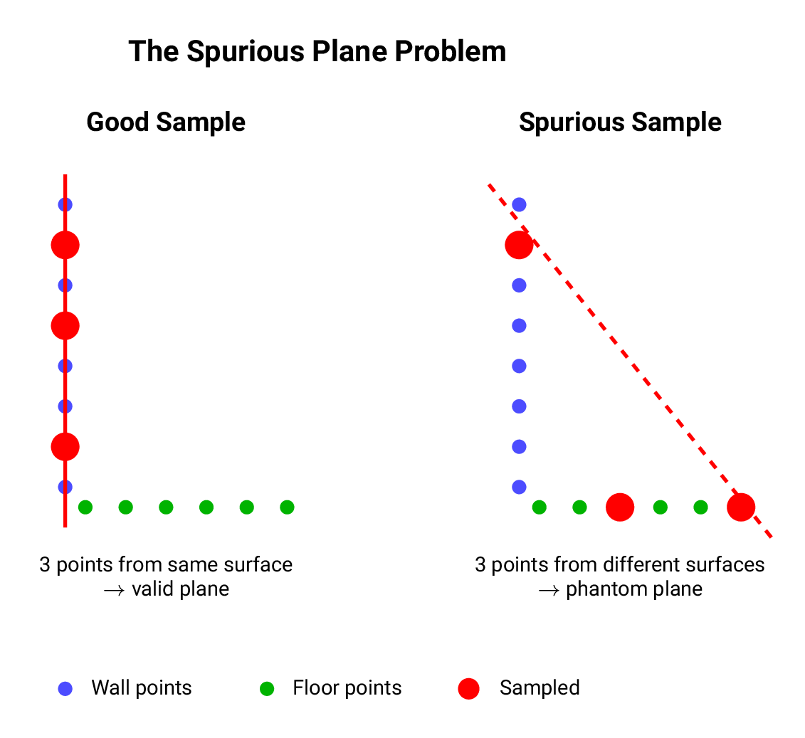{fig-cap="Left: sampling 3 points from the same wall yields a valid plane. Right: sampling from wall AND floor yields a diagonal phantom plane that doesn't exist."}
## NDT-RANSAC: Eliminating Spurious Planes
I implemented NDT-RANSAC based on Li et al. [@li2017].
**NDT (Normal Distribution Transformation)** fixes the spurious planes problem by pre-classifying regions of space into planar and non-planar cells. Instead of sampling 3 random points, we sample from locally planar regions.
### Step 1: Classify Cells by Shape using NDT
The algorithm voxelizes space and computes statistics for each cell:
```{python}
#| label: ndt-cell
@dataclass
class NDTCell:
"""
A cell in the Normal Distribution Transform grid.
Eigenvalue shape classification (sorted λ₁ ≤ λ₂ ≤ λ₃):
- Planar: λ₁ << λ₂ ≈ λ₃ (λ₁/λ₂ ≤ threshold) → flat surface
- Linear: λ₁ ≈ λ₂ << λ₃ (λ₂/λ₃ ≤ threshold) → edge/line
- Spherical: λ₁ ≈ λ₂ ≈ λ₃ → noise or point feature
"""
indices: np.ndarray # Point indices belonging to this cell
centroid: np.ndarray # Mean position (3,)
normal: np.ndarray # Eigenvector of smallest eigenvalue
eigenvalues: np.ndarray # Sorted: λ₁ ≤ λ₂ ≤ λ₃
is_planar: bool # True if λ₁/λ₂ ≤ planarity_threshold
is_linear: bool = False # True if λ₂/λ₃ ≤ linearity_threshold
def compute_cell_features(points: np.ndarray) -> tuple:
"""Compute NDT features for a group of points."""
centroid = np.mean(points, axis=0)
centered = points - centroid
# Covariance matrix
cov = np.dot(centered.T, centered) / len(points) # <1>
# Eigendecomposition (returns sorted ascending)
eigenvalues, eigenvectors = np.linalg.eigh(cov) # <2>
eigenvalues = np.abs(eigenvalues)
# Normal = eigenvector of smallest eigenvalue
normal = eigenvectors[:, 0] # <3>
normal = normal / (np.linalg.norm(normal) + 1e-10)
# Planarity test: λ₁/λ₂ ≤ threshold
planarity_threshold = 0.04
if eigenvalues[1] < 1e-10:
is_planar = False
else:
is_planar = (eigenvalues[0] / eigenvalues[1]) <= planarity_threshold
return centroid, normal, eigenvalues, is_planar
# Demo with synthetic planar points
np.random.seed(42)
# Points on a plane z = 0 with small noise
planar_pts = np.column_stack([
np.random.uniform(-1, 1, 100),
np.random.uniform(-1, 1, 100),
np.random.normal(0, 0.01, 100) # Small z-noise
])
centroid, normal, eigenvalues, is_planar = compute_cell_features(planar_pts)
print(f"Eigenvalues: {eigenvalues}")
print(f"Ratio λ₁/λ₂: {eigenvalues[0]/eigenvalues[1]:.4f}")
print(f"Is planar: {is_planar}")
print(f"Normal: {normal} (should be ~[0, 0, 1])")
```
1. Covariance matrix captures the spread of points in each direction
2. `eigh` returns eigenvalues sorted ascending - important for our ratios
3. The smallest eigenvalue's eigenvector points perpendicular to the spread
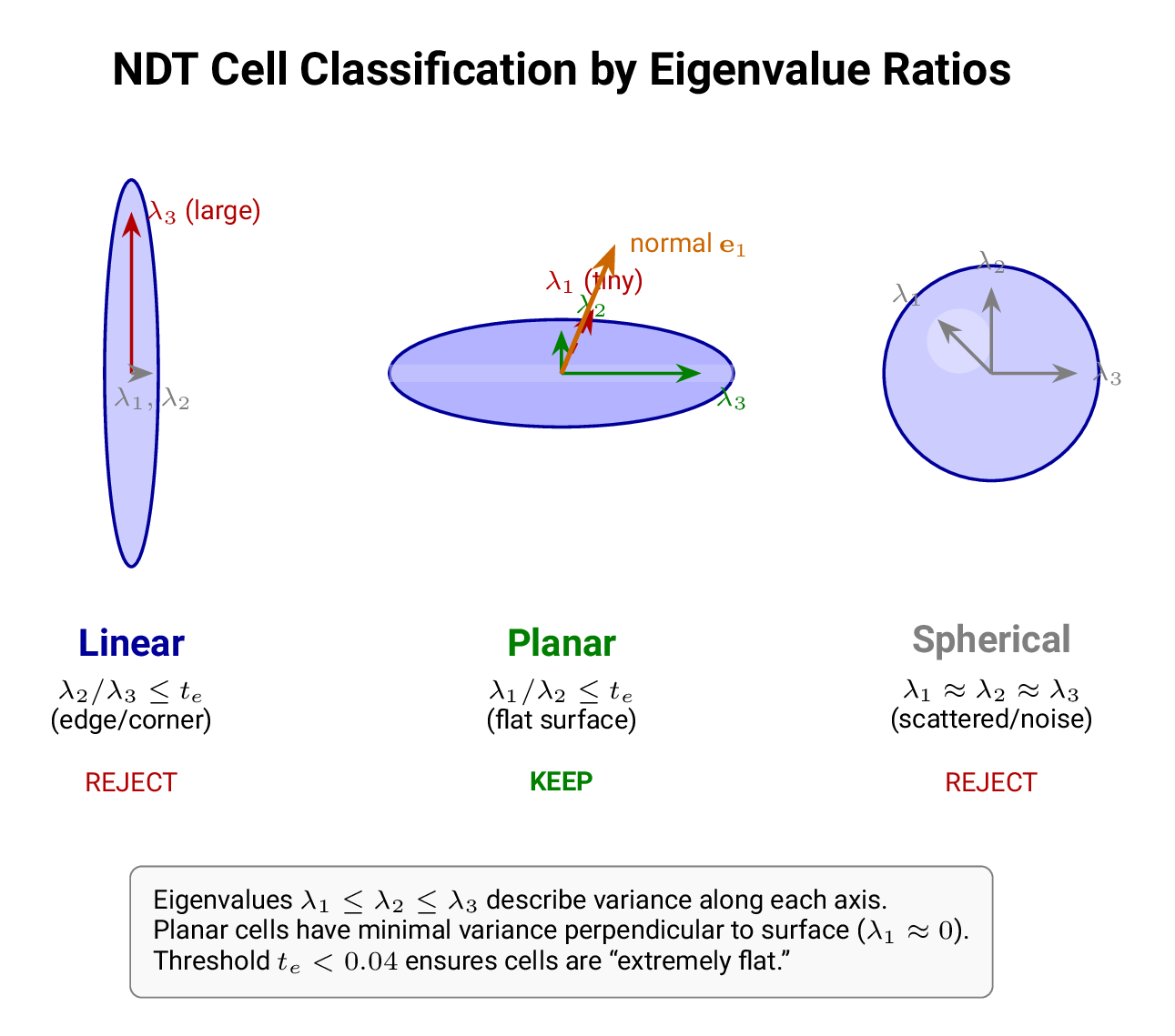{fig-cap="The eigenvectors are the principal axes (directions), and the eigenvalues are the magnitudes. Together they describe how points spread within each cell."}
::: {.callout-note}
If you're familiar with basic statistics but not linear algebra: the covariance matrix is just the multi-dimensional version of variance. We are effectively fitting a 3D Gaussian distribution, hence the name **Normal Distribution Transformation**.
:::
### The Key Insight: Better Sampling Probability
**Because we sample from pre-classified planar cells, the probability of picking a good sample is dramatically improved**:
| Method | P(good sample) | w = 10% |
|--------|---------------|---------|
| Standard RANSAC | $w^3$ | 0.1% per iteration |
| NDT-RANSAC | $w$ | 10% per iteration |
That's a 100× speedup: instead of hoping 3 random points all land on the same surface, you pick one cell that's *already proven* to be planar.
### Step 2: Grow the Plane
Selecting a good seed cell is only the first step. We need to find all other cells belonging to the same plane using a **dual condition**:
1. **Spatial Proximity**: Distance from cell center to the hypothesized plane < $\Delta_d$
$$d = |(\mathbf{g}_{cell} - \mathbf{g}_{seed}) \cdot \mathbf{n}_{seed}|$$
2. **Normal Consistency**: Angle between cell normal and plane normal < $\Delta_\theta$
$$\theta = \arccos(\mathbf{n}_{cell} \cdot \mathbf{n}_{seed})$$
Typical thresholds from the paper: $\Delta_d = 0.08m$, $\Delta_\theta = 15°$.
### Step 3: Refine with IRLS
After finding inliers, we need to fit the final plane equation. Standard least-squares minimizes $\sum r_i^2$ where $r_i$ is each point's distance to the plane. The problem: **outliers have outsized influence**.
**IRLS (Iteratively Reweighted Least Squares)** fixes this by iteratively adjusting weights:
$$\text{minimize} \sum w(r_i) \cdot r_i^2$$
```{python}
#| label: irls-fit
def irls_fit_plane(
points: np.ndarray,
max_iter: int = 10,
convergence_threshold: float = 1e-6
) -> tuple[np.ndarray, np.ndarray]:
"""
Robust plane fitting using IRLS with Welsch weight function.
w(r) = exp(-r²/k²) where k = 2.985
"""
k_welsch = 2.985 # Standard tuning constant for 95% efficiency # <1>
# Initial fit via SVD
centroid = np.mean(points, axis=0)
centered = points - centroid
_, _, vh = np.linalg.svd(centered)
normal = vh[-1]
normal = normal / np.linalg.norm(normal)
for iteration in range(max_iter):
old_normal = normal.copy()
# Compute residuals (distances to plane)
residuals = np.abs(np.dot(centered, normal))
# Welsch weights: exp(-r²/k²)
weights = np.exp(-(residuals ** 2) / (k_welsch ** 2)) # <2>
# Weighted centroid
weighted_centroid = np.average(points, axis=0, weights=weights)
centered = points - weighted_centroid
# Weighted covariance
weighted_cov = np.dot(centered.T * weights, centered) / weights.sum()
# New normal from smallest eigenvalue
eigenvalues, eigenvectors = np.linalg.eigh(weighted_cov)
normal = eigenvectors[:, 0] # <3>
normal = normal / np.linalg.norm(normal)
centroid = weighted_centroid
# Check convergence
if np.max(np.abs(normal - old_normal)) < convergence_threshold:
break
return normal, centroid
# Demo: plane with outliers
np.random.seed(42)
# Main plane: z ≈ 0
inliers = np.column_stack([
np.random.uniform(-2, 2, 80),
np.random.uniform(-2, 2, 80),
np.random.normal(0, 0.05, 80)
])
# Outliers: points far from plane
outliers = np.column_stack([
np.random.uniform(-2, 2, 20),
np.random.uniform(-2, 2, 20),
np.random.uniform(1, 3, 20) # Way off the plane
])
points_with_outliers = np.vstack([inliers, outliers])
# Compare standard vs IRLS
standard_normal, _ = np.linalg.svd(points_with_outliers - points_with_outliers.mean(axis=0))[2][-1], None
standard_normal = standard_normal / np.linalg.norm(standard_normal)
irls_normal, irls_centroid = irls_fit_plane(points_with_outliers)
print(f"True normal: [0, 0, 1]")
print(f"Standard LS normal: {np.abs(standard_normal).round(3)}")
print(f"IRLS normal: {np.abs(irls_normal).round(3)}")
```
1. The value $k = 2.985$ achieves 95% efficiency - losing only 5% precision vs standard LS when there are no outliers
2. Welsch weights fall off exponentially with distance, effectively ignoring far outliers
3. After reweighting, we solve the normal eigenvalue problem again
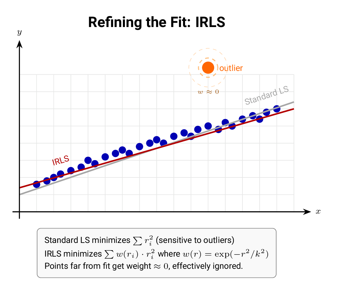{fig-cap="Standard least squares (gray line) gets pulled toward the outlier. IRLS (red line) downweights distant points, producing a fit that matches the actual data distribution."}
::: {.callout-tip}
If you've used `glm()` in R, you've used IRLS - it's the algorithm that fits generalized linear models internally.
:::
### Step 4: Handle Disconnected Components
After fitting a plane, we need to handle an additional problem: **a mathematical plane is infinite, but physical surfaces are finite**.
RANSAC might find a single plane that contains points from two disconnected physical walls if they share the same orientation and both satisfy the distance threshold.
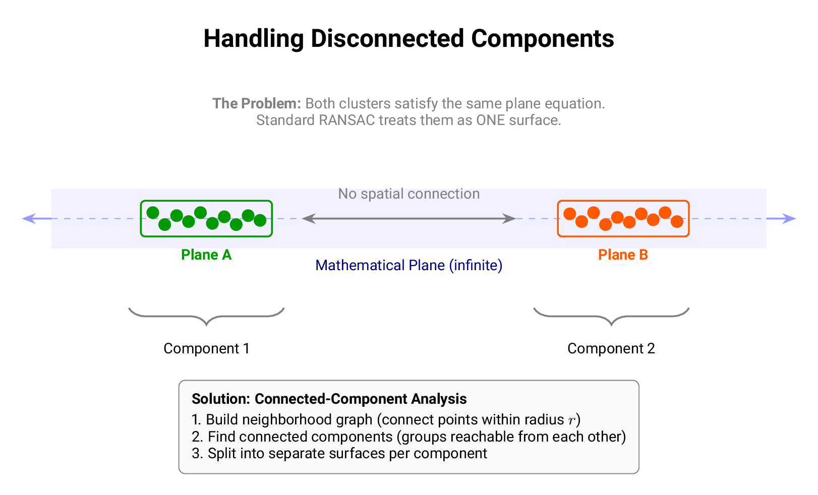{fig-cap="The \"teleportation problem\": A single mathematical plane (light blue, infinite) can intersect two separate physical walls. Without connected-component analysis, RANSAC would treat these as one surface."}
**Connected-component analysis** solves this by examining spatial connectivity:
```{python}
#| label: connected-components
from scipy.spatial import KDTree
from scipy.sparse import csr_matrix
from scipy.sparse.csgraph import connected_components
def split_by_connectivity(
inlier_points: np.ndarray,
neighbor_radius: float = 0.1,
min_component_points: int = 50
) -> list[np.ndarray]:
"""
Split points into spatially connected groups.
Args:
inlier_points: (N, 3) points on a detected plane
neighbor_radius: Max distance for connectivity (2-3× RANSAC threshold)
min_component_points: Filter small components as noise
"""
n_points = len(inlier_points)
if n_points < min_component_points:
return [np.arange(n_points)]
# Build KD-tree for neighbor queries
tree = KDTree(inlier_points)
# Find all neighbor pairs within radius
pairs = tree.query_pairs(r=neighbor_radius, output_type='ndarray') # <1>
if len(pairs) == 0:
return [np.arange(n_points)] # No connections
# Build sparse adjacency matrix
row_indices = np.concatenate([pairs[:, 0], pairs[:, 1]])
col_indices = np.concatenate([pairs[:, 1], pairs[:, 0]])
data = np.ones(len(row_indices), dtype=np.int8)
adjacency = csr_matrix(
(data, (row_indices, col_indices)),
shape=(n_points, n_points)
)
# Find connected components
n_components, labels = connected_components( # <2>
adjacency, directed=False, return_labels=True
)
# Split into groups
groups = []
for comp_id in range(n_components):
mask = labels == comp_id
if mask.sum() >= min_component_points:
groups.append(np.where(mask)[0])
return groups if groups else [np.arange(n_points)]
# Demo: two separate clusters
np.random.seed(42)
cluster1 = np.random.randn(100, 3) * 0.1 + [0, 0, 0]
cluster2 = np.random.randn(100, 3) * 0.1 + [5, 0, 0] # 5m away
combined = np.vstack([cluster1, cluster2])
groups = split_by_connectivity(combined, neighbor_radius=0.3, min_component_points=20)
print(f"Found {len(groups)} connected components")
for i, g in enumerate(groups):
center = combined[g].mean(axis=0)
print(f" Component {i+1}: {len(g)} points, center at {center.round(2)}")
```
1. `query_pairs` efficiently finds all point pairs within radius using the KD-tree
2. `connected_components` is the same algorithm used in image processing to identify blobs
## The Real Challenge: Boundary Extraction
Detecting planes was the easy part. The difficult part was turning detected wall planes into a clean boundary polygon.
### Ceiling-Height Filtering
First problem: **we're detecting too many wall segments**. Many "wall" segments are actually furniture - bookcases, cabinets, and other vertical surfaces that happen to be planar.
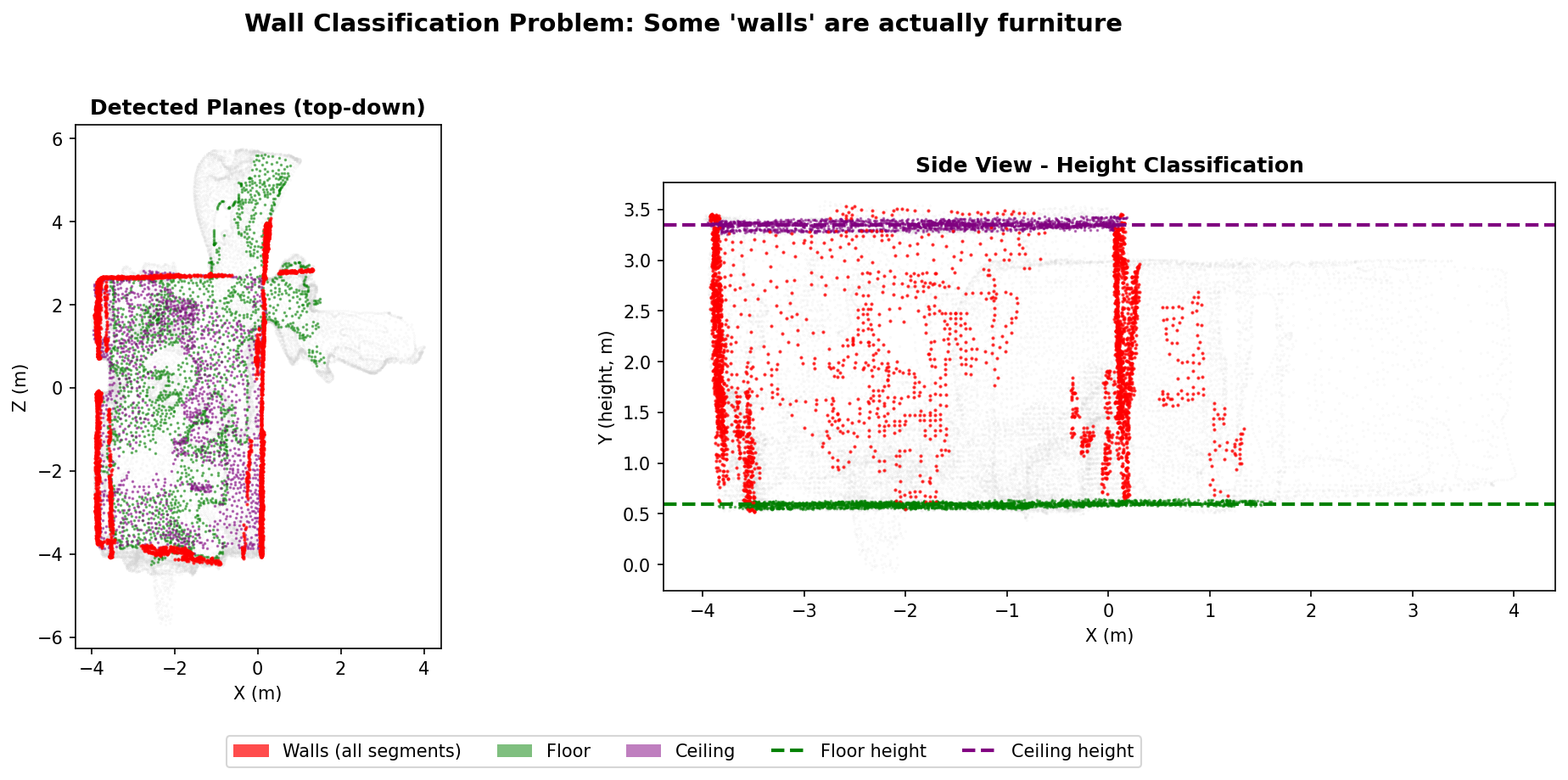{fig-cap="The problem: All red segments are classified as \"walls\" by RANSAC. But look at the side view (right) - many segments stop well below the ceiling line. These are furniture, not walls."}
**Filtering by height**: Keep only segments where `y_max >= 2.0m`. This simple threshold eliminates most furniture while keeping all true walls.
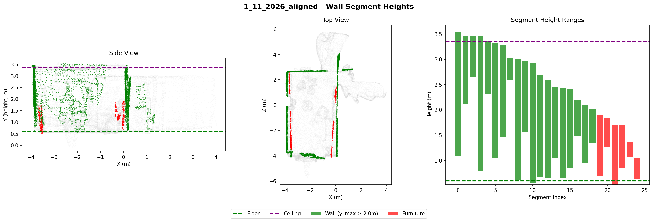{fig-cap="Left: Side view showing wall segments (green) reaching ceiling vs furniture (red) stopping mid-height. Middle: Top-down view confirms walls form the perimeter while furniture is interior. Right: Bar chart showing the clear 2.0m threshold separating walls from furniture."}
### Enclosure Filtering: Handling Doorways
Height filtering removes furniture, but there's another problem: **doorways**. The scanner captured points through open doors into hallways and adjacent rooms. These points pass the height filter (hallway walls also reach the ceiling), but they're not part of the room we're trying to extract.
The solution is **enclosure scoring** - a ray-casting algorithm that identifies which regions are "inside" vs "outside" the room:
```{python}
#| label: enclosure-filtering
#| code-fold: true
#| code-summary: "Show enclosure scoring algorithm"
def compute_enclosure_score(
    x: float, z: float,
    wall_segments: list[tuple],
    ray_directions: list[tuple] = [(1, 0), (-1, 0), (0, 1), (0, -1)]
) -> int:
    """
    Count how many ray directions hit a wall.

    A point is "enclosed" if rays in multiple directions hit walls.
    """
    hits = 0
    for dx, dz in ray_directions:
        # Cast ray and check for wall intersections
        # (simplified - real implementation checks segment bounds)
        for seg_start, seg_end in wall_segments:
            if ray_intersects_segment(x, z, dx, dz, seg_start, seg_end):
                hits += 1
                break  # One hit per direction is enough
    return hits

def ray_intersects_segment(x, z, dx, dz, start, end):
    """Check if ray from (x,z) in direction (dx,dz) hits segment."""
    # Parametric ray-segment intersection
    x1, z1 = start
    x2, z2 = end

    # Ray: (x,z) + t*(dx,dz), t >= 0
    # Segment: (x1,z1) + s*(x2-x1,z2-z1), 0 <= s <= 1

    denom = dx * (z2 - z1) - dz * (x2 - x1)
    if abs(denom) < 1e-10:
        return False  # Parallel

    t = ((x1 - x) * (z2 - z1) - (z1 - z) * (x2 - x1)) / denom
    s = ((x1 - x) * dz - (z1 - z) * dx) / denom

    return t >= 0 and 0 <= s <= 1
```
The algorithm:
1. **Create a 2D grid** over the XZ projection (0.3m cells)
2. **For each cell**, cast rays in 4 cardinal directions (N, S, E, W)
3. **Count wall hits**: How many rays intersect a detected wall segment?
4. **Score the cell**: Cells with walls on multiple sides (score ≥ 2) are "enclosed"
5. **Find largest region**: Use connected-component analysis to identify the main room
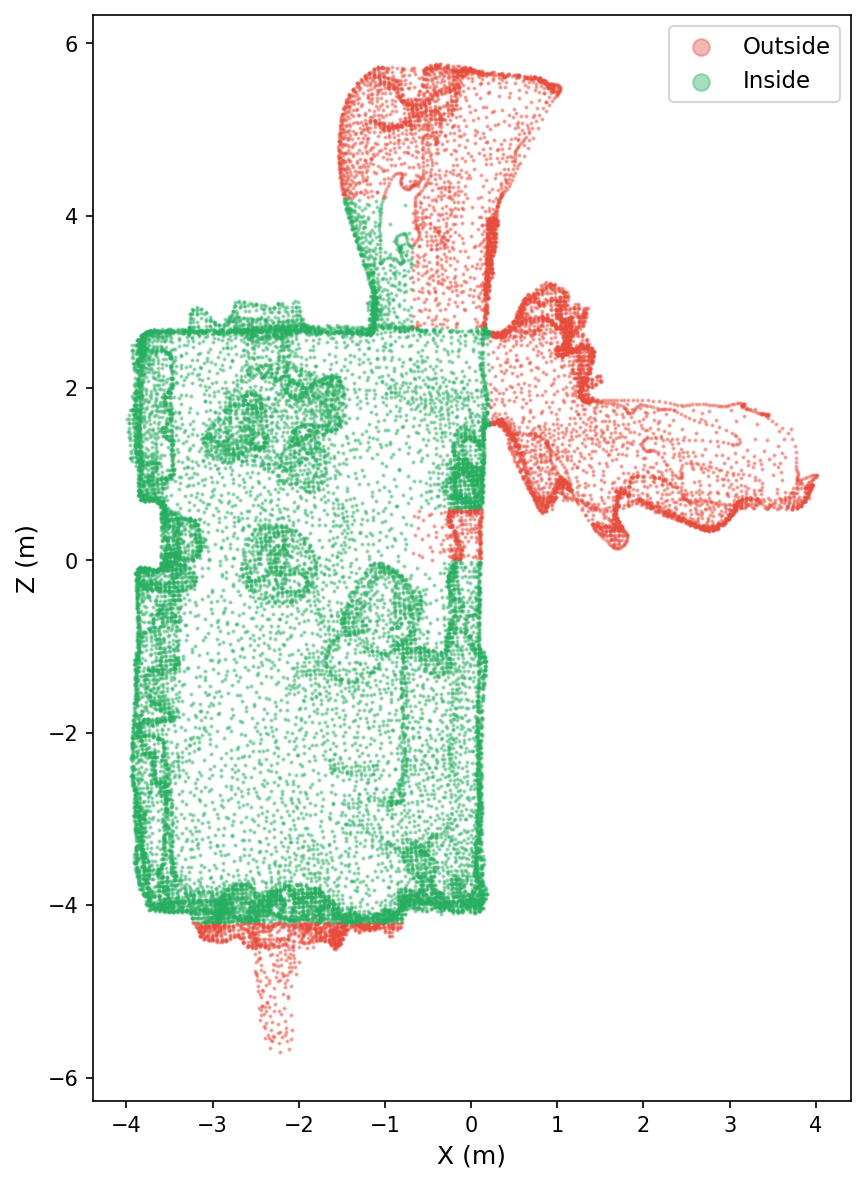{fig-cap="Enclosure filtering in action. Green points are \"inside\" - enclosed by walls on multiple sides. Red points are \"outside\" - the hallway through the doorway (right), an adjacent room (top), and areas where walls weren't detected (bottom)."}
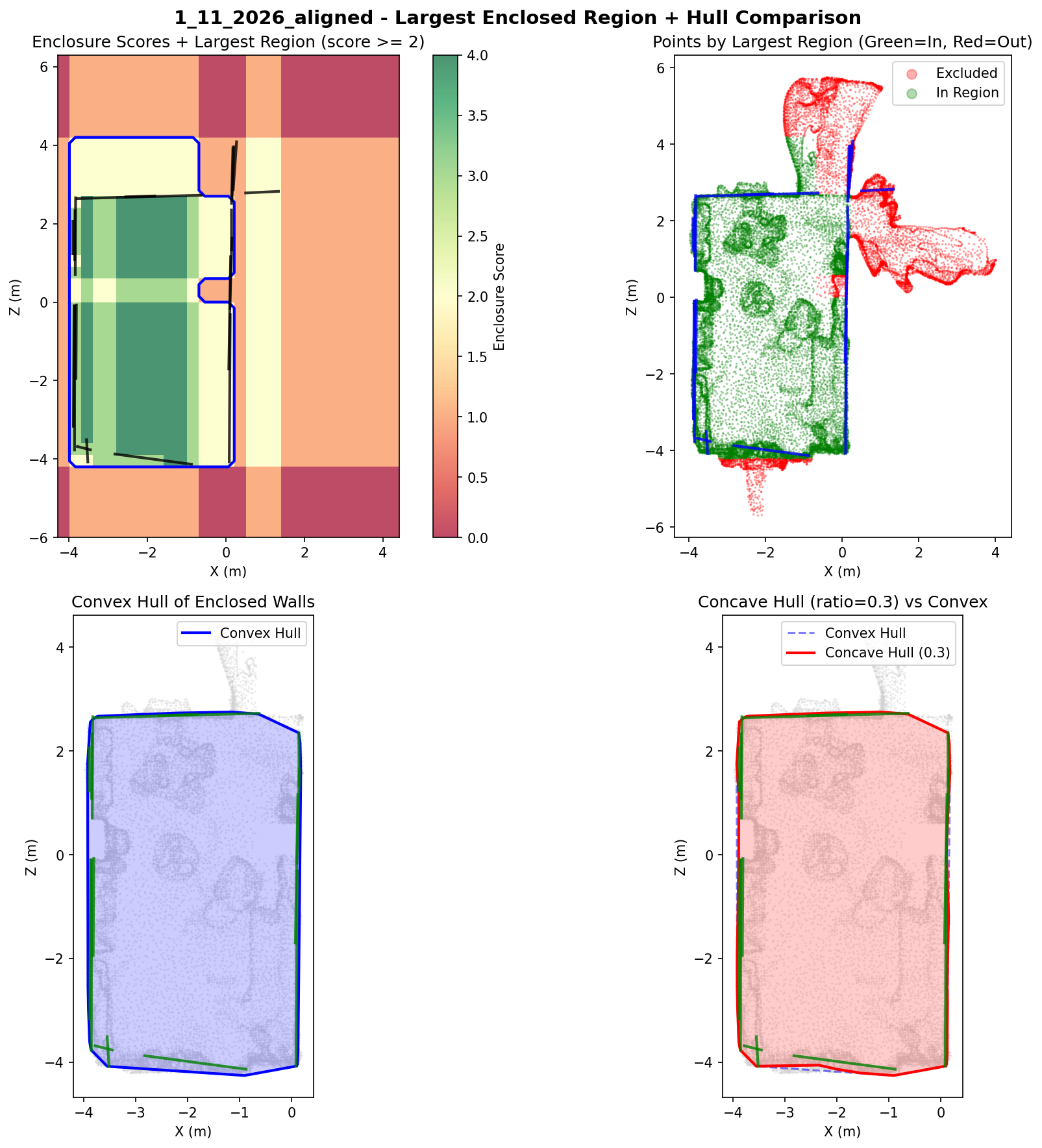{fig-cap="Enclosure filtering visualization after alignment (version 2)."}
## Edge Detection: Beyond Planes
The same eigenvalue analysis that identifies planar cells can identify **linear** cells (edges). For linear cells, $\lambda_2/\lambda_3 \leq 0.2$ - points spread along one dominant direction while the perpendicular spreads are similarly small.
Edges provide information planes cannot: **room corners** (vertical edges where walls meet) and **missing wall inference** (edge exists but no plane detected → unscanned wall).
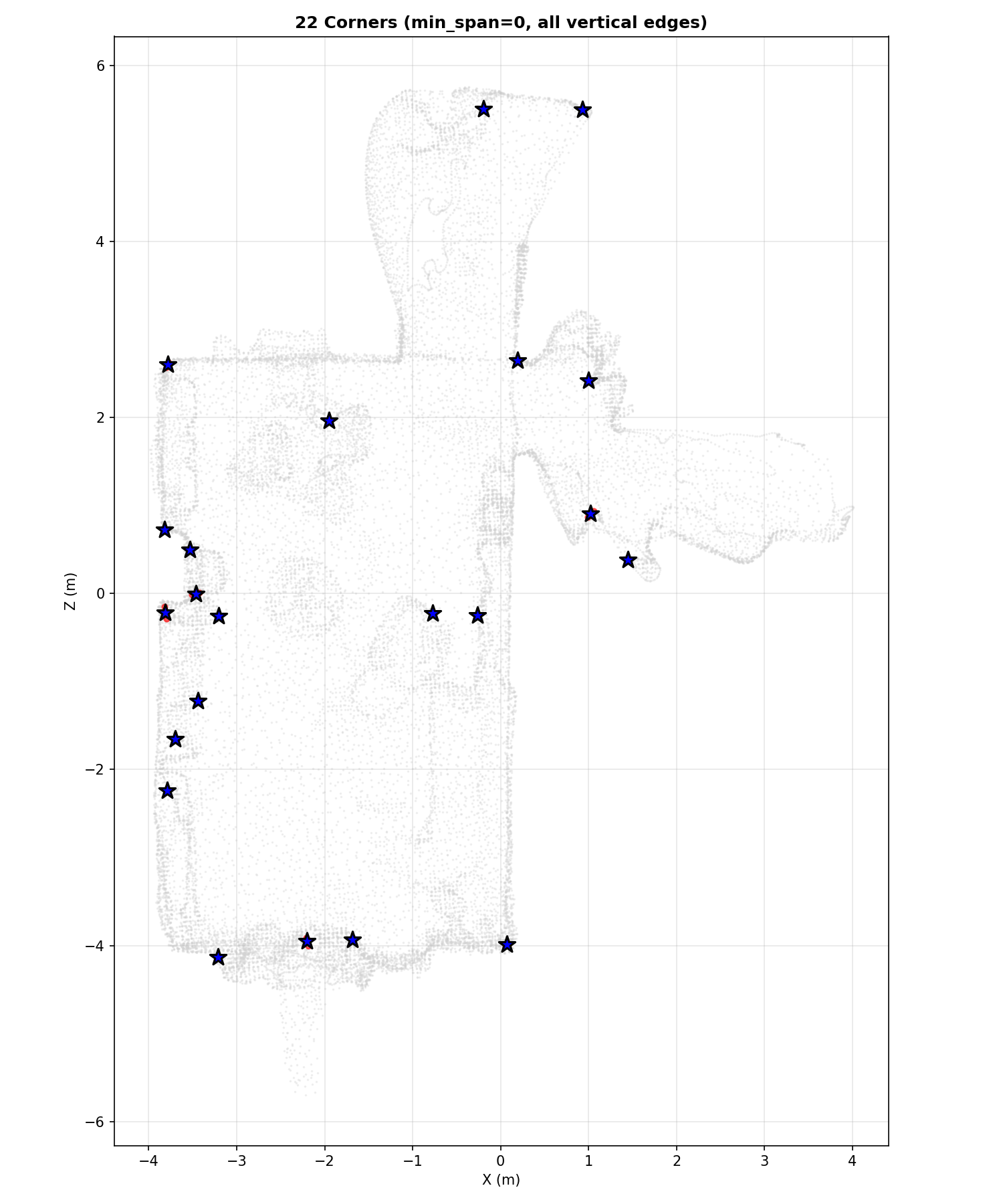{fig-cap="Vertical edge cells (red dots) classified as \"linear\" with vertical direction. Clustering by XZ position reveals 22 corner candidates (black stars). Many align with obvious room corners; some mark furniture edges."}
## Tuning the Cell Size
The theoretical constraint from Li et al. [@li2017]:
$$\left(\frac{\varepsilon}{s}\right)^2 < t_e < 0.04$$
Where $\varepsilon$ = sensor noise, $s$ = cell size, $t_e$ = planarity threshold.
The cell must be large enough that noise doesn't dominate eigenvalue spread. Too small: noise overwhelms geometry, everything looks "spherical". Too large: misses detail, merges distinct surfaces.
### Mesh Density Varies Wildly
| Mesh | Density (pts/m²) |
|------|------------------|
| 1_11_2026_aligned.obj | **291** |
| Untitled_Scan.obj | **835** |
| 1_11_2026_4.obj | **1,298** |
A 4× density difference between scans of the same apartment.
**Practical rule**: sparse phone photogrammetry needs 25-50cm cells; dense TLS can use 10-25cm.
## Next Steps
The CCW ordering failure points to a fundamental issue: we're trying to construct a complex polygon from unordered corners. With the ceiling-height filter reducing noise, several alternative approaches to explore:
1. **Convex hull + selective inward refinement**: Start with the simplest valid boundary (convex hull of wall points), then selectively "push in" edges only where strong evidence of indentation exists.
2. **Grid-based occupancy**: Discretize the floor into a 2D grid, mark cells containing wall points, then trace the boundary using marching squares.
3. **Constrained concave hull**: Use a concave hull algorithm (alpha shapes) but constrain edges to align with detected Manhattan directions.
4. **Boundary tracing**: Instead of finding all corners then ordering them, start at one segment and "walk" the perimeter - always turning to the next adjacent segment.
The perfect room boundary extractor remains elusive, but each iteration reveals more about the problem structure. The key insight: **start simple, add complexity only where data supports it**.
## Lessons Learned
1. **Real-world data is messy.** Furniture occludes walls, scanning artifacts create phantom planes, doorways create gaps that may or may not be intentional room boundaries.
2. **NDT pre-classification is powerful.** By reasoning about local geometry before sampling, we eliminate entire classes of errors.
3. **Connected components matter.** A mathematical plane can span disconnected physical surfaces - always check spatial connectivity.
---
## References










